Generic LJ Simulator in OpenMM

I present a script and JSON input file for building and running complex Lennard-Jones particle mixtures in 2D and 3D in a variety of conditions using OpenMM.

The 12-6 Lennard-Jones (LJ) potential.

The Lennard-Jones potential model is a very simple model that most-accurately describes the interactions of Noble gas elements. The Lennard-Jones potential defines the interaction between two atoms separated by distance \(r\):

\(U(r) = 4 \epsilon \left[ \left(\frac{\sigma}{r}\right)^{12} - \left(\frac{\sigma}{r}\right)^{6} \right]\).

The positive term, \(4 \epsilon \left(\frac{\sigma}{r}\right)^{12}\) approximates the Pauli exclusion of electron-electron interactions (at short distance). The negative term, \(-4 \epsilon \left(\frac{\sigma}{r}\right)^{6}\), approximates the instantaneous dipole attraction between atoms; the London dispersion force. Each part of the potential and their sum look like this:
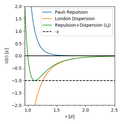
Figure The 12-6 Lennard-Jones potential (green) and its’ constituent parts.

The simplicity of this model is very attractive for exploring general concepts in physics. Many coarse-grained force fields mostly consist of atoms described using Lennard-Jones potentials with harmonic potentials describing their connectivity. Particles described using only the Lennard-Jones potential are often called “Lennard-Jones particles”.

Reduced units of the Lennard-Jones model.

In thinking about real systems, we need units to understand the relative size and scale of all things. Energies we often express in units like kJ/mol, temperatures in K, volumes in nm³, et cetera. However, if a system is simple enough, it is easy to express thermodynamic quantities in terms of each other, such that all quantities are unitless, but can be related directly back to real, unit-having values, which can describe many systems a la the Theorem of corresponding states. This idea that we can understand many real systems via studying systems using reduced units is another reason why Lennard-Jones simulations can be attractive for exploring new ideas.

To perform MD simulations, it is necessary to define parameters like the time step, temperature, density. For equilateral systems of (\(d\)) dimensions, the temperature (\(T\)), density (\(\rho\)), integration time step \(\tau\), and langevin damping coefficient \(\gamma\) are defined as:

Real Quantity	Conversion from Reduced Quantity (*)
\(T\)	\(\ k_B/ \epsilon^* T^*\)
\(\rho\)	\(N \sigma^{*d} / \rho^*\)
\(\tau\) (MD time step)	\(\sqrt{ m^* \sigma^{*2} / \epsilon^*}\)
\(\gamma\) (Damping coefficient)	\(\tau/2\)

The reduced \(\epsilon\), \(\sigma\), and mass (\(m\)), for these equations use the weighted average of these quanitites for each \(i^{th}\) LJ particle type relative to their ratio of system composition (\(\alpha_i\)), out of \(M\) particle types:

Weighted Average of Reduced Quantity	Definition
\(\left< \sigma^* \right>\)	\(\sum_i^M \alpha_i \sigma_i\), \(\ \ \ \ \ \ \ \ \ \ \alpha_i = n_i / \sum_i^M n_i\)
\(\left< \epsilon^* \right>\)	\(\frac{1}{M} \sum_i^M \sum_j^M \epsilon_{ij} \alpha_i\)
\(\left< m^* \right>\)	\(\sum_i^M \alpha_i m_i\)

There is another, not so general reduced unit we use to think about conditions for phase separation in binary mixtures that is available as an input for this LJ simulator. In Flory-Huggins models the energetic cost of forming lattice contacts with a lattice site of differing type is expressed by the parameter \(\chi\). The reduced unit in these models is then expressed as the ratio \(\frac{k_B T^*}{\chi}\). We can define \(T\) in our simulations using a these reduced units, too, to perform LJ simulations to explore theories developed in such simple theoretical models or lattice simulations.

Quantity	Definition
\(\chi_{int}\)	\(-\epsilon_{12} - \left( \frac{-\epsilon_{11} - \epsilon_{22}}{2} \right)\)
\(T^*\)	\(\frac{k_B T^*}{\chi_{int}} \frac{\chi_{int}}{k_B}\)
\(T\)	\(\ \epsilon^* T^* / k_B\)

In this case we refer to this as \(\chi_{internal}\), as the Flory-Huggins theory parameter \(\chi\) is meant to fold in the contrubutions from entropy, and thus there is some difference between the results of the LJ model and Flory-Huggins theory at this value of \(\chi\).[1]

A few example simulations.

I’ve made a little set of scripts that make it very easy to run Lennard-Jones particle simulations in OpenMM using a simple input script. The script LJ_simulation.py takes care of building the system using Packmol, setting up the system in OpenMM, and handling two- and three-dimensional molecular dynamics simulations of these systems. It can run any number of different types of Lennard-Jones particles in any proportion, with the option of two different initial conditions. It outputs all information in reduced units, using the hacked up reducedstatedatareporter.py.

Here are a few examples.

A simulation with M=2, N=2000, where \(\epsilon_{11}^*\) = \(\epsilon_{22}^*\) = 4, \(\epsilon_{12}^*\) = \(\epsilon_{21}^*\) = 0.4, \(\sigma_1^*\) = \(\sigma_2^*\) = 1, \(m_1^*\) = \(m_2^*\) = 1, \(T^*\) = 1, \(\rho^*\) = 0.75, and \(d\) = 2 and the system composition is at 50% type 1, and 50% type 2, running for 50,000,000 steps (at a rate of approx. 60,000,000 steps / hour on a GTX 2080 super), initiated from a mixed state:

The above simulation could also be defined using \(\frac{k_B T^*}{\chi_{int}}\) = 2.3096 as the user input, rather than \(T^*\) = 1.

A simulation with \(M\)=3, \(N\)=1000, where \(\epsilon_{11}^*\) = \(\epsilon_{12}^*\) = \(\epsilon_{21}^*\) = \(\epsilon_{22}^*\) = \(\epsilon_{23}^*\) = \(\epsilon_{32}^*\) = \(\epsilon_{33}^*\) = \(\epsilon_{13}^*\) = \(\epsilon_{31}^*\) = 1, \(\sigma_1^*\) = \(\sigma_2^*\) = \(\sigma_3^*\) = 1, \(m_1^*\) = \(m_2^*\) = \(m_3^*\) = 1, \(T^*\) = 2, \(\rho^*\) = 0.8, and \(d\) = 3 and the system composition is at 40% type 1, 40% type 2 and 20% type3, running for 200,000 steps, initiated from a stripe-shaped phase separation:

A simulation with \(M\)=3, \(N\)=1000, where \(\epsilon_{11}^*\) = \(\epsilon_{12}^*\) = \(\epsilon_{21}^*\) = \(\epsilon_{22}^*\) = \(\epsilon_{23}^*\) = \(\epsilon_{32}^*\) = \(\epsilon_{33}^*\) = \(\epsilon_{13}^*\) = \(\epsilon_{31}^*\) = 1, \(\sigma_1^*\) = \(\sigma_2^*\) = \(\sigma_3^*\) = 1, \(m_1^*\) = \(m_2^*\) = \(m_3^*\) = 1, \(T^*\) = 2, \(\rho^*\) = 0.8, and \(d\) = 3 and the system composition is at 40% type 1, 40% type 2 and 20% type3, running for 200,000 steps, initiated from a stripe-shaped phase separation. Now including an external potential to restrain particles to the stripe phase with widthscale = 0.95 and kwall = 20 (this potential is described later):

A bit about OpenMM: What makes it nice for quickly exploring ideas and what can make it difficult to use.

OpenMM uses SWIG to generate C++ code from strings at the python API level to define custom potentials and integrators, and to modify simulation parameters during simulation. OpenMM also supports reading of the matured MD force field parameter file formats of CHARMM, AMBER, and GROMACS. This makes it possible to use OpenMM as a testbed for development of creative simulation methods by using simple models that can later be scaled up to production simulations. It also makes it possible to create totally new simulation methods that can be used without recompiling OpenMM.

Sometimes, understanding how to write strings that will be correctly interpreted by OpenMM to do what you want can be difficult, so I will present how I do that for this LJ simulator as another example of how to use OpenMM. Reading the C++ code is the most sure-fire way to really get an idea of what to do at the python level if it’s not clear.

For example, to accomplish two-dimensional simulations I needed to:

1. Create a custom velocity verlet langevin integrator (LJ_simulation.py)
2. Add a new integrator variable that is the Vec3 vector <1,1,0> (LJ_simulation.py)
3. Multiply all velocities by this new <1,1,0> vector when determining displacement, and later before determining kinetic energy (LJ_simulation.py)
4. Re-define the instantaneous temperature to account for the missing dimension in kinetic energy when printing output (reducedstatedatareporter.py)

But I had not seen a demonstration of how to do steps 1-3 anywhere, so I had to determine what to do by reading how variables are defined in the C++ program openmmapi/include/CustomIntegrator.h in the OpenMM source (not distributed with the conda installation – see the github) Step 4 was straightforward because it does not rely on interpreting and compiling a string.

Constructing a pair-interaction-specific Lennard-Jones potential in OpenMM.

A pretty flexible Lennard-Jones model should be able to adopt different interactions strengths between different types of Lennard-Jones particle. We want to be able to freely define how different LJ interaction energies will be formed between each \(i^{th}\) and \(j^{th}\) atom type, \(\epsilon_{ij}\). The user is able to define this in the “epsilonAR_r” section of the JSON input file. We could also freely define how different LJ interaction lengths (\(\sigma_{ij}\)) are formed, but we should stick with something more sane in this case, and apply the standard Lorentz combination rule to determine the \(\sigma_{ij}\) parameters from each particle’s radius described by \(\sigma_i\).

Here, the array epsilonAR_r and the list sigmas_r correspond to the first example simulation, which has \(M\)=2 particle types:

# epsilons are in reduced units, kJ/mol in OpenMM (i.e. 1.0 = epsilon, 2.0 = 2epislon)
epsilonAR_r = np.array([
[4.0, 0.4], #eps1-1, eps1-2
[0.4, 4.0], #eps2-1, eps2-2
], dtype="float64")
sigmas_r = [1.0, 1.0] # LJ sigmas in reduced units in order of particle type, nanometers in OpenMM
sigmaAR_r = np.zeros((M,M), dtype="float64")
for i in range(M):
    for j in range(i,M):
        sigmaAR_r[i][j] = np.true_divide(sigmas_r[i]+sigmas_r[j],2.0)
        sigmaAR_r[j][i] = sigmaAR_r[i][j]

# the Lennard-Jones potential we will create in OpenMM accepts these arrays in list form
epsilonLST_r = (epsilonAR_r).ravel().tolist()
sigmaLST_r   = (sigmaAR_r).ravel().tolist()

We now want to add a nonbonded force to the system that describes how all types of LJ particle interact. We can write out the standard 12-6 LJ potential, but with terms that describe specific pairs of atom types, a feature which is enabled by using the expressions “eps=epsilon(type1, type2)” and “sig=sigma(type1, type2)”…

print('Constructing OpenMM simulation')
system = mm.System()
system.setDefaultPeriodicBoxVectors(mm.Vec3(box_edge_r, 0, 0), mm.Vec3(0, box_edge_r, 0), mm.Vec3(0, 0, box_edge_r))
customNonbondedForce = mm.CustomNonbondedForce('4*eps*((sig/r)^12-(sig/r)^6); eps=epsilon(type1, type2); sig=sigma(type1, type2)')
customNonbondedForce.setNonbondedMethod(mm.NonbondedForce.CutoffPeriodic)
customNonbondedForce.setCutoffDistance(min(box_edge_r*0.49*u.nanometers, cutoff_r*u.nanometers))
customNonbondedForce.addTabulatedFunction('epsilon', mm.Discrete2DFunction(M, M, epsilonLST_r))
customNonbondedForce.addTabulatedFunction('sigma', mm.Discrete2DFunction(M, M, sigmaLST_r))
customNonbondedForce.addPerParticleParameter('type')

After that we need to tell every particle to use this force, then add the force to the system.

# set the particle parameters
particle_index = 0
for alpha in range(M):
    for i in range(particle_index, particle_numbers[alpha] + particle_index):
        system.addParticle(masses_r[alpha]*u.amu)
        customNonbondedForce.addParticle([alpha])
        particle_index += 1
system.addForce(customNonbondedForce)

Disabling changes to the z-axial positions to achieve two-dimensional simulations.

OpenMM does not support two-dimensional simulations, however we can create a custom integrator that ignores the z-axis in computing velocity-related quantities, like displacement in the z-dimension and the z-dimension contribution to the kinetic energy. There are a few examples of how to make and manipulate custom integratiors within the comments of openmmapi/include/openmm/CustomIntegrator.h in the OpenMM source.

To do this, a “dummy” variable, a Vec3 Vector of <1,1,0> needs to be created. This is used to multiply the velocities of each atom to remove z-axis kinetic energy. This also disables displacements into the z-dimension. I call this variable “dumv”.

if dimensions == 2:
    integrator.addPerDofVariable("dumv", 1.0) # makes a <1,1,1> vector
    integrator.setPerDofVariableByName("dumv", [mm.Vec3(x=1.0, y=1.0, z=0.0)])

In the custom integrator, we’ll multiply the velocity of each atom by “dumv” (<1,1,0>) to remove z-axial displacements.

if dimensions == 2: # To get a 2D system, make z-velocities zero when moving x
    integrator.addComputePerDof("x", "x + v*dumv*dt")
else:
    integrator.addComputePerDof("x", "x + v*dt")

The resulting velocities from each step of integration will be multiplied by “dumv” to remove the z-axial contribution to the kinetic energy.

if dimensions == 2: # Remove the resulting z-velocities to get the correct Kinetic Energy
    integrator.addComputePerDof("v", "v*dumv")

This is not quite everything that needs to be done. In two-dimensional systems the integrator will run just fine at a reference temperature of \(T^{*}\), but the reported instantaneous temperature will be off by 2/3. This is corrected in the hacked up “ReducedStateDataReporter” class that is imported from “reducedstatedatareporter.py”.

Creating a periodic external potential to restrain particles to stripe phases.

Phase separations that form in the thermodynamic limit can become unstable at insufficient system sizes given a system temperature and the interaction cost for forming contacts between species of opposites type. We explored this idea in lipid bilayers and an analytical two-dimensional Flory-Huggins lattice model in 2017.[2] Simulating lipid bilayers that should phase separate, but will not phase separate at the small system sizes required to run sufficiently fast simulations in MD, can be biased to remain in a phase separated state by effectively creating a “wall” using a flat-well harmonic potential. Park and Im recently applied such a flat-well potential to stabilize a phase separations of POPC-DPPC and DOPC-DPPC binary lipid bilayers including unrestrained cholesterol to determine the partition coefficient of cholesterol to either phase.[3] We express this potential with the equation

\(U_{\mathrm{wall}}(x) = k_{\mathrm{wall}} \max\left(0, \mid x - x_0 \mid - (w \times \mathrm{widthscale}) \right)^2\),

where \(x_0\) is the center of a stripe phase, \(w\) is the radius of the restraint from the center, widthscale is a scaling factor on \(w\), and \(k_{\mathrm{wall}}\) is the biasing force.

Here is an illustration:

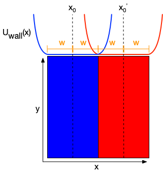
Figure: Flat well potential effectively creating a soft wall enforcing a phase separation in an equimolar binary mixture.

This flat-well potential can be expressed in the following form in OpenMM:

flatres = mm.CustomExternalForce('forcewall * (px^2); \
                               px = max(0, delta); \
                               delta = r - droff; \
                               r = abs(periodicdistance(x, y, z, x0, y, z));')
flatres.addGlobalParameter('forcewall', forcewall)
flatres.addGlobalParameter('droff', width)
flatres.addPerParticleParameter('x0')

where periodicdistance is a special function in CustomExternalForce that enforces distances are measured over the PBC. Without this, particles will fly from one side of the box to the other once passing through the PBC. It would be easy to change this potential to restrain “dot” phases too.

Parameters of the JSON input file.

To easily run Lennard-Jones simulation with reduced units in OpenMM, the script LJ_simulation.py, which loads reducedstatedatareporter.py to record thermodynamic quantities and build systems using Packmol can be controlled externally using JSON input files which are loaded as a command line argument.

For example 1, we run use the following JSON file as an input “python LJ_simulation.py ex1.json”

{
"pdb_prefix": "ex1",
"dcd_prefix": "ex1",
"nc_prefix": "ex1",
"data_name": "ex1.dat",

"initial_condition": "mixed",
"N": 2000,
"T_r": 1,
"density_r": 0.75,
"dimensions": 2,
"particle_ratios": [1, 1],
"sigmas_r": [1, 1],
"masses_r": [1, 1],
"epsilonAR_r": [
        [4, 0.4],
        [0.4, 4]
        ],

"numsteps":         50000000,
"data_interval":       10000,
"coordinate_interval": 10000,
"frcvel_interval":     10000,
"platform_type": "CUDA",

"minimization": false,
"restraint_widthscale": 1.0,
"forcewall": 10.0,
"enable_restraint": false
}

• “pdb_prefix” is the name prefix of .pdb files from system construction and minimization
• “dcd_prefix” is the name prefix of a .dcd file containing the simulation trajectory
• “nc_prefix” is the name prefix of a .nc NetCDF file containing the simulation velocities and forces (Optional)
• “data_name” is the name of an output text file written from ReducedStateDataReporter. This also names a .tcl script for quickly loading a rudimentary visualization in VMD.
  
• “initial_condition” set Packmol to construct either a randomly-mixed or phase-separated initial condition
• “N” the total number of particles in the system
• “T_r” the reduced temperature
• “density_r” the reduced density
• “dimensions” the number of dimensions (2 or 3)
• “particle_ratios” the relative ratio of each particle type, in any proportion. This gets normalized later.
• “sigmas_r” the reduced Lennard-Jones \(\sigma\) of each particle type
• “masses_r” the reduced mass of each particle type
• “epsilonAR_r” the reduced, pair-type-specific Lennard-Jones \(\epsilon\)s
• “numsteps” the number of MD steps to perform
• “data_interval” thermodynamic quantities and simulation progress recorded during simulation
• “coordinate_interval” the coordinate writing frequency (.dcd file)
• “frcvel_interval” the force and velocities writing frequency (.nc file; Optional)
• “platform_type” choice of computation platform. CUDA, OpenCL, or CPU
  
• “minimization” turns minimization on/off with booleans “true”/”false”
• “restraint_widthscale” scales width of the flat-well restraint (1=edge-to-edge of the initial stripe phase), if enabled
• “forcewall” kwall flat-well restraint
• “enable_restraint” turn the flat-well restraint on/off with the booleans “true”/”false”. Might explode if simulation is initiated from “initial_condition”: “mixed”

As mentioned earlier, LJ_simulation.py can also take temperature defined via \(\frac{k_B T^*}{\chi_{int}}\) instead of \(T^*\). This can be done by defining “kbT_chi instead of “T_r”. An example of this is given in ex1-kbT_chi.json.

LJ_simulation.py can take restart files as inputs and write them as outputs after simulation. These are controlled by the optional, additional parameters “rstin_prefix” and “rstout_prefix”, which name these files without an extension.

LJ_simulation.py can also optionally not save the NetCDF file containing positions, forces, and velocities. If you don’t want this, or want to save space, you can choose to not define “nc_prefix” and “frcvel_interval”.

One warning: I do not suggest using minimization. For two-dimensional systems minimization can move particles along the z-axis, and I do not think it is possible to correct this behavior without modifiying code that would need to be recompiled. Additionally, Packmol does a good job of constructing the system, so minimization should not be necessary in three-dimensional systems either.

Precompiled OpenMM can be installed using conda (I suggest using Miniconda). I strongly suggest reading the User manual and following the instructions to set up CUDA if you have a NVIDIA GPU. Parmed is requiredto write the NetCDF .nc file containing forces and velocities, which can also be installed with conda. Packmol is easy to compile. JSON can be installed using conda, too. You need to set the path to Packmol on your local computer in LJ_simulator.py for the variable “path_to_Packmol”.

The python scripts that perform these simulations are available on my github at https://github.com/gpantel/MD_methods-and-analysis/blob/master/LJsimulator, in addition to input files to perform these three example simulations.

References:

1. Chremos, A., Nikoubashman, A. & Panagiotopoulos, A. Z. Flory-Huggins parameter χ, from binary mixtures of Lennard-Jones particles to block copolymer melts. J. Chem. Phys. 140, 1–10 (2014).
2. Pantelopulos, G. A., Nagai, T., Bandara, A., Panahi, A. & Straub, J. E. Critical size dependence of domain formation observed in coarse-grained simulations of bilayers composed of ternary lipid mixtures. J. Chem. Phys. 147, 095101 (2017).
3. Park, S. & Im, W. Quantitative Characterization of Cholesterol Partitioning between Binary Bilayers. J. Chem. Theory Comput. 14, 2829–2833 (2018).